
Bleeding An Ensemble Sort
After blogging about the possibility of beating Java sort performance, I got really obsessed to prove my case with integers.
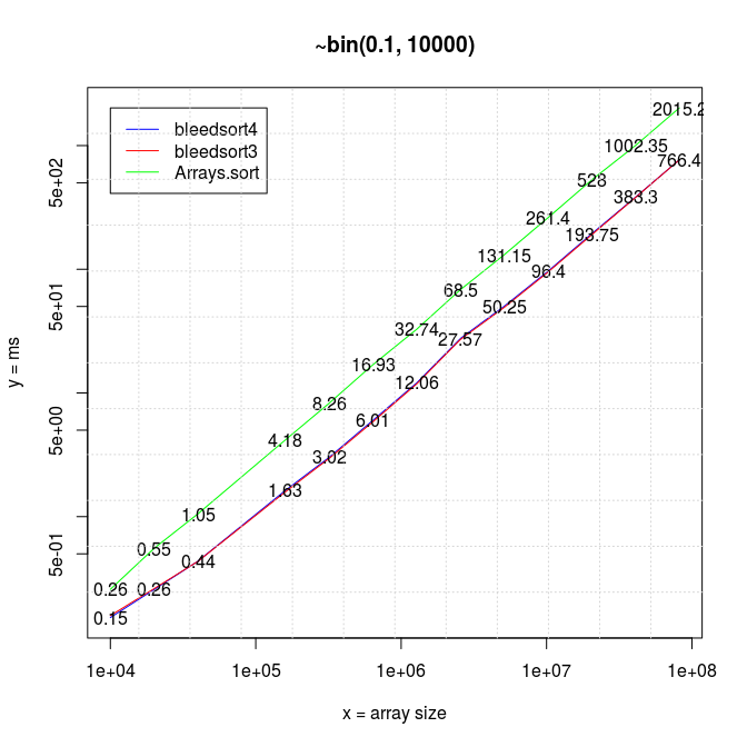
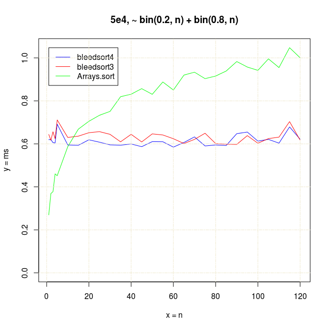
To start where I left in the earlier post, below is a series of plots of binomial benchmarks that the first version of bleedsort did so poorly on. (plots: R).
Starting from my earlier code, I created new versions of bleedsort 2 3 4 4b 5, and ran quick benchmarks on them with different datasets. If you look at the benchmarks 3 3-2 4 4b 4b-2 5, there are many kinds of errors and biases in them. My results indicate that a great deal can be done towards a robust general intelligence for sorting large arrays. These are not perfectly accurate measurements. What I wanted was quick insight into my developing algorithms, not a solid record of value. More thorough data could be gathered later if I succeeded well enough.
I have 20*x (x≥1) measurements for each data point in all pictures.
Benchmarks: fallibility and other concerns
As of earlier I was running benchmarks with JMH. It is an established microbenchmark framework backed by the expertise of Oracle’s engineers. But I couldn’t test as much and as fastly as I needed to with it. My algorithms evolved very quickly and a JMH run for a single datapoint could take an hour or more if data was hard to prepare. I wrote versions 3 and 4 of bleedsort on two successive days to contrast with. I tried to shorten my sampling times, but the results then had blatant variance. Also JMH enforced some restrictions in building supportive structures, recycling data, etc.
I switched away to hand-written JUnit benchmarks. JUnit is more tightly integrated with my IDE, which also was nice for explorative testing.
The binomial charts illustrate a very Java-like fault that ensued – I found JUnit times varying hugely over days. I run on two different machines, but it had nothing to do with that. What was I not noticing?
I was benchmarking three algorithms against same data in successive loops. This was very nice for ad hoc analysis (I could track down performance issues to the exact form of random data when I needed to), but running different things together allows them affect each other.
Because small datasets are very fast to sort, I had created extra weight by measuring 20*x rounds of sorting instead of 20. Now when I ran bleedsort3 x times, then bleedsort4 x times, then Arrays.sort x times, repeat, I found bleedsort performance degrade sharply with some data sizes and some x.
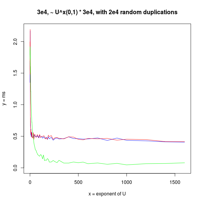
It felt natural to guess that my benchmarks collided badly with the gc cycle. Bleedsorts as distribution sorts do make relatively large ad hoc memory reservations. They were also the sorts that were slowing down, whereas Arrays.sort had much less variance. This could be like 100% slowdown in a bad case. There is a blue datapoint at array size 4e4 in the last picture that illustrates this. I could repeat performance degradation simply by re-running a test with specific parameters, so it was not totally random.
I tried driving gc by hand, but it only made things weird. However varying the number of inner-loop executions seemed to modify the degradation pattern, even to the point of removing degradation. Arrays.sort times remained more stable throughout.
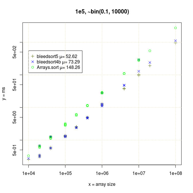
Now by some manual variation I could find a nice cycle for each measurement. I switched away from plotting lines (breaking that fun illusion of continuity) and started plotting individual datapoints.
(This all could be methodized as a search over cycle space, which is perhaps one of the things that JMH does under the hood.)
My JUnit tests do some priming too, not as correct as in JMH, I’m sure, but it helps a little anyway.
I’ll explain my algorithms shortly and then we’ll get to the graphs.
Algorithm-specific sampling techniques
I was a bit misleading to speak about bleedsort, since my sort turned into an orchestrated ensemble of sort strategies.
From bleedsort3 upwards, my sorts sample a target array in not one but many ways.
For bleedsorts, as distribution sorts, the amount of repetition in an array is a key question. A relatively unique array will map neatly on a scale, but if there are many densely packed places and duplicate items, bleedsorts will plunge to suboptimal pit.
This is why I needed to estimate the amount of repetition found in a dataset. My original idea was to take twenty patches of 100 items from the target array and calculate average repetition per value from this sample. It was not enough.
I needed to sample also longer runs of 1/4 array size. The short runs had relatively low likelihood of hitting duplicates in large arrays.
All this sampling means that I can not compete with sorting small or already sorted arrays. So I’m not doing that, as stated before. As a teaser however I wrote a naive monotonous mergesort that beats Arrays.sort when sorting sine waves of small frequences.
The second thing that I sampled was quite naturally data distribution. In bleedsort1 I started with three quantiles, 0th, 50th, and 100th. This of course meant a very bad estimate for many kinds of data. In bleedsort2 I used five quantiles 0, 25, 50, 75, and 100. In bleedsort3 I switched to nine quantiles 0, 12.5, 25, … , 100 and have stuck with them since.
I sample a batch of 160 random items from the array and order them to get nine quantile estimates. They provide some fast solutions for algorithm choice. They are also used by bleedsorts.
Algorithms
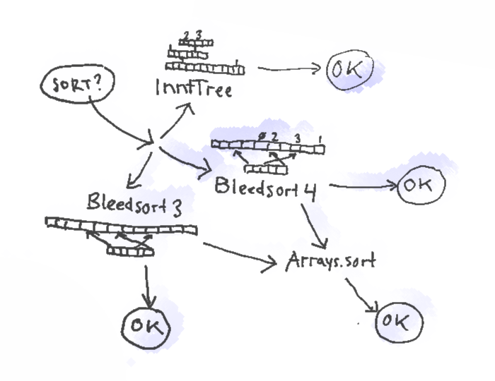
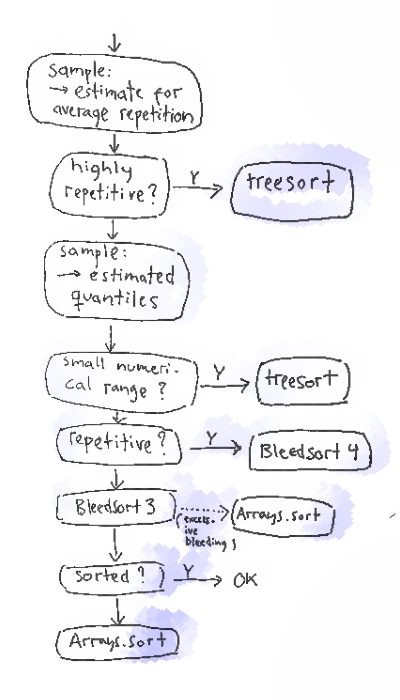
Here’s a picture of the sort paths of the bleedsort4 ensemble.
Bleedsort3/4 themselves are distribution sorts based on 9 quantiles that map to eight buckets in temporary space. Bleedsort4 is a counting sort, and it uses half of its temporary space for storing item counts, whereas bleedsort3 moves items around individually. Both have runtime heuristics to terminate execution when they run to trouble. Trouble for them means too dense items, making them bleed and slow down. It means that they can leave an array to a halfway sorted state with the mentality “OK, I’m sorry but I couldn’t do more now”. They then delegate their work from that state on to another algorithm.
In the code, I tried to keep sampling as cost-effective as possible, but standard library sort performance is still much better with small target arrays. This is due to an initial cost brought by sampling and of course because Java library sorts are quite robust. With larger arrays, the cost of sampling gets gradually insignificant and its benefits start to weigh more.
Bleedsort4 and 3 are explained above.
InntTree
is a tailored ordered static-depth counting tree
with O(1) puts and gets within “theoretical clean complexity”, not taking
memory management into account. Iteration is not O(1) but it is still in practise
very fast. InntTree is robust in some problems but must be used with some caution.
A big and evenly spread data range increases
memory costs and slows down both storage and retrieval.
As a variation I also implemented SmallRangeInntTree, which has even more flat a structure with only two node levels and autoexpanding array buckets to keep memory footprint initially as low as possible.
The following flow chart gives a more detailed explanation of sampling and selection in bleedsort4.
Data
I describe here what kinds of distributions and arrangements I tested so far. I refrained to sorting 32 bit signed integers, as said, which enables me to use common statistical methods while poking the data. It means that bleedsort could be extended to longs (64 bit int) and floating point numbers, but not to arbitrary objects, in particular never to objects that only implement the Java interface Comparable but do not possess more powerful properties for mapping to a linear space (ascii strings, for instance, could be mapped in base 128 by their 4 first digits).
I must stress that these benchmarks are very tricky with respect to extrapolating trends, so I would not recommend that.
I also have insufficient records of what code path is responsible for each result. The decision is nowadays stored by the benchmark script, but it was not when I ran some of these benchmarks.
Binomial distributions
My first mission was to get binomial distributions very fast. There is a normal distribution near to a binomial distribution with sufficiently large values of n, so binomial performance correlates with normal performance. This makes binomial distributions nice to be good at.
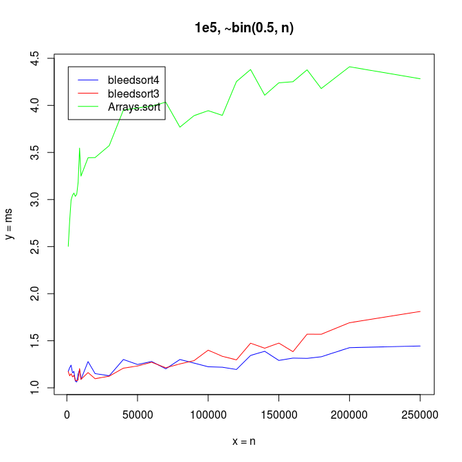
My main result is graph 1 plotted earlier, and some supplementary benchmarks follow.
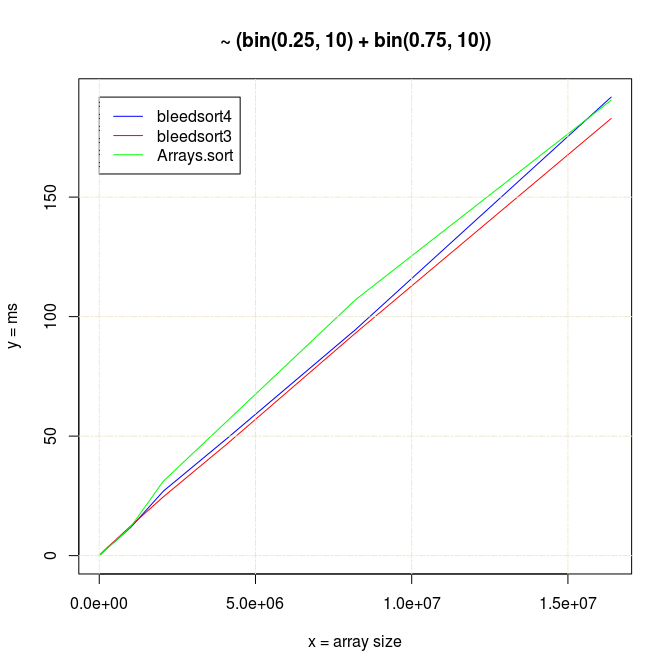
Bleedsort performance is very good and also degrades more slowly than that of Arrays.sort when the binomial base n increases (illustrated in the following picture). Bleedsort4 slope is especially favorable towards large n’s. Array size remains 100,000 throughout the following benchmarks:
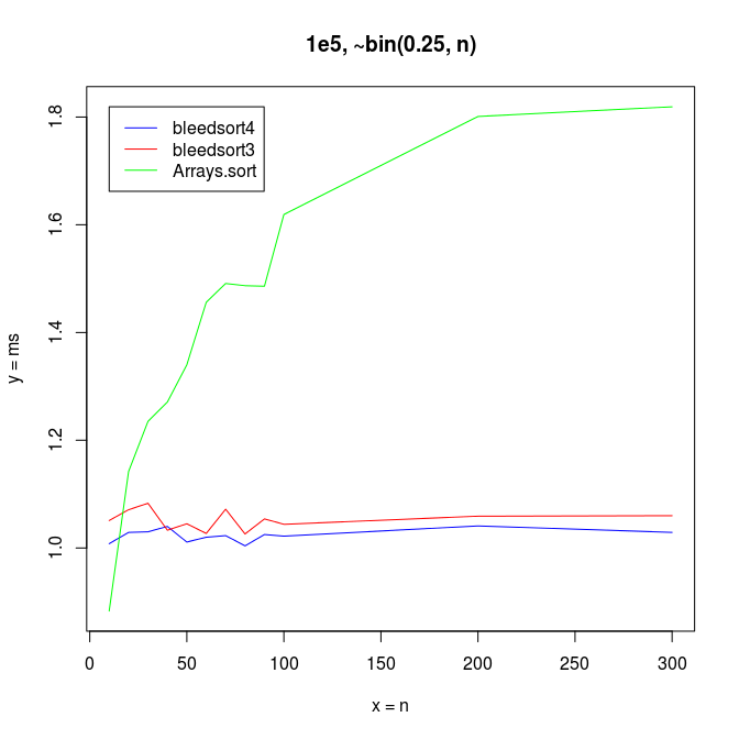
With small n’s and array size 100,000, Arrays.sort dominates up to n=15, but bleedsorts give more constant performance when n grows:
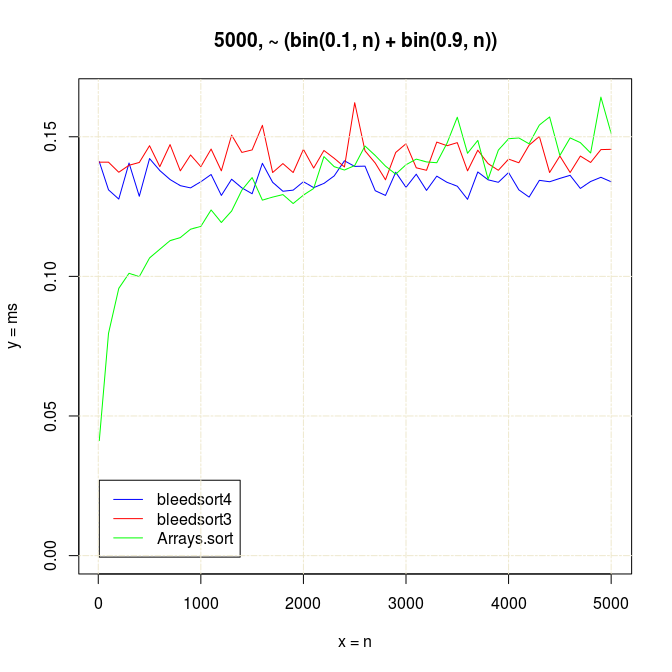
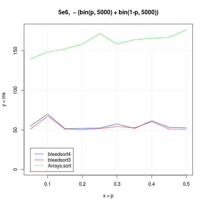
To get a feel for slightly more difficult data, I benchmarked some bimodal binomial distributions.
Already with small arrays of 5000 items with
n growing, Arrays.sort starts to slow down in comparison with more constantly performing
bleedsorts. Arrays.sort seemed faster on these
bin(p,n)+bin(1-p,n) when n < 3000 and array size < 10000:
With somewhat larger arrays bleedsorts start to win with much smaller n’s, around n=15:
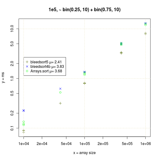
Sort times of big binomial arrays can be three to four times faster with bleedsorts than with Arrays.sort, when n is moderately big.
On the other hand when n is very small (array consists of a few distinct values like in the following example), Arrays.sort performs better than bleedsorts or nearly same.
Wishing to compete with this I covered some new special cases in the decision phase of Bleedsort5 (which slightly degraded performance in some other problems).
It is an interesting fact to note that Arrays.sort (quicksort) finds a de-centered bimodal distribution easier to sort than a cluttered one, at least when data is randomly placed:
Of course, quicksort performance was also degrading when binomial n was increasing, illustrated earlier.
Uniform distributions
Uniform distributions are easy to generate (with the exception of super-uniform data…). Sorting might be needed with 3D scenes or other spatially or temporally ordered series of events.
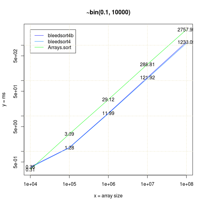
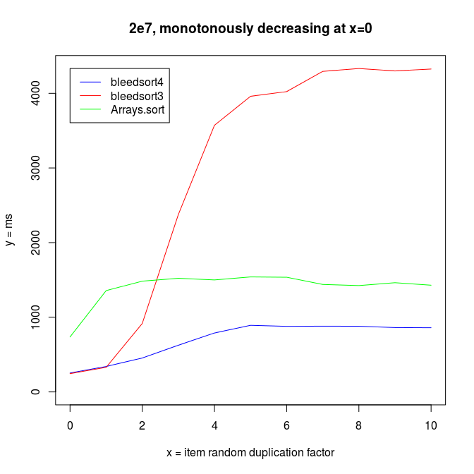
Bleedsort performance seemed competitive up to 2e7 arrays, but then something strange happened:
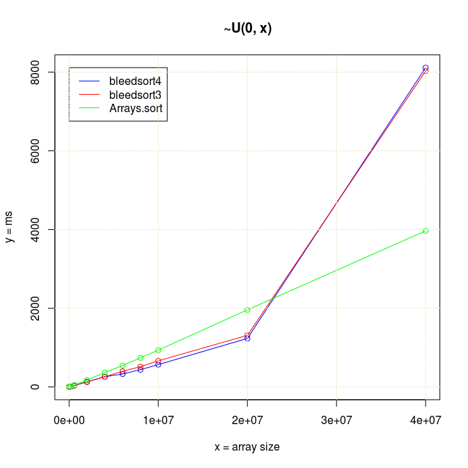
Actually there is a bug in sampling code that was frozen for Bleedsort4. I made a fix for this in 4b and tested it a little in 5 (graph not available).
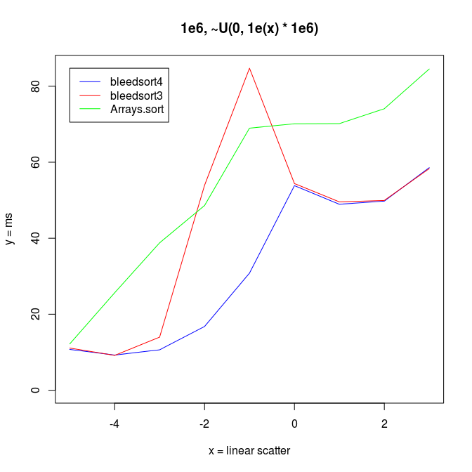
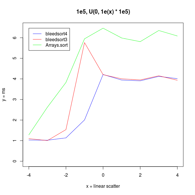
Following two charts show how when U distributes over a wide range, bleedsort4 heuristics shines over bleedsort3 and Arrays.sort:
Next I wanted to vary the simple uniform distribution to make it appear more like some real datasets.
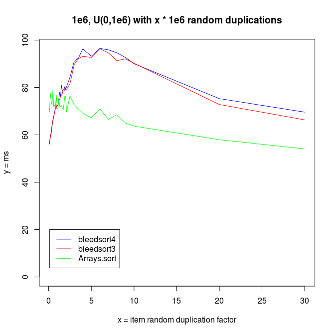
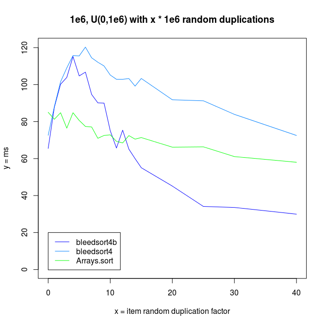
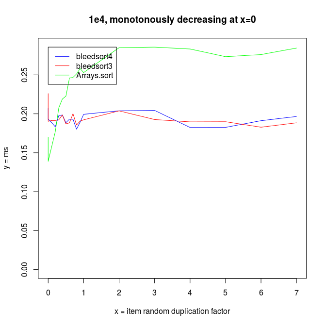
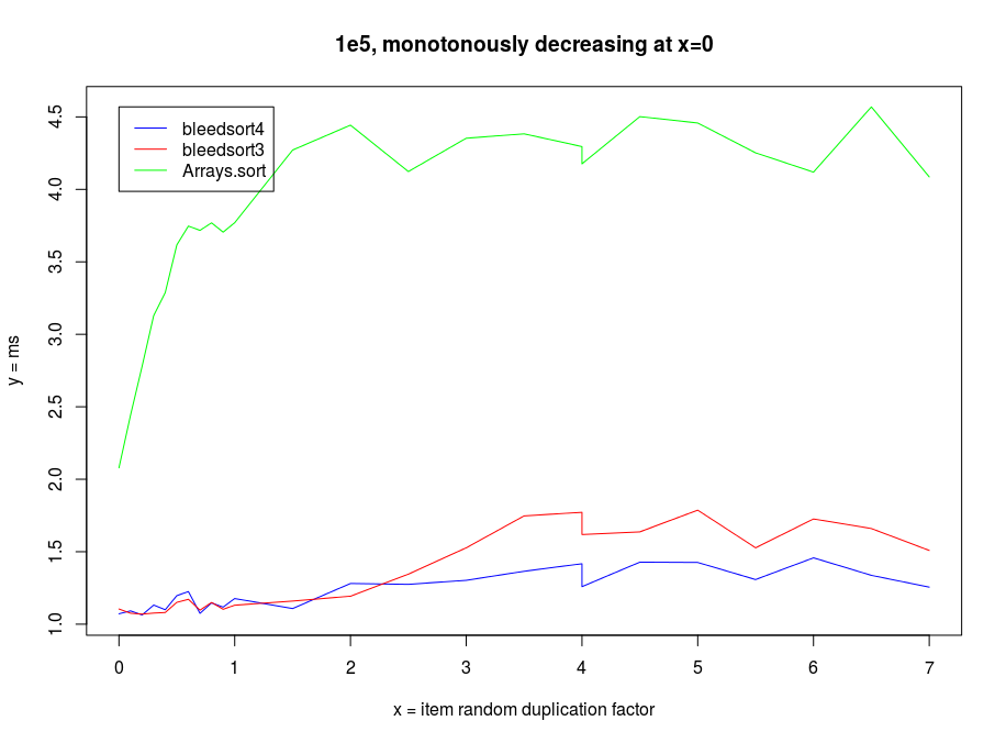
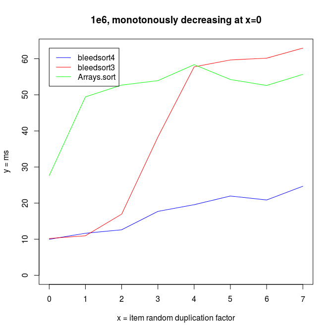
I increased redundancy in test distributions, replacing items by randomly chosen source items from the same array. This increases repetition in the array.
In these kinds of problems, Arrays.sort won clearly over bleedsorts. I analyzed this a bit and found that it is a sampling problem. Bleedsort could pick another sort strategy, but signs of repetition are lost into the haystack of a big array. For this I created the longer sampling runs described in an earlier section.
It is interesting to note that both bleedsorts and quicksort (Arrays.sort) start to perform better, when data reduplication increases.
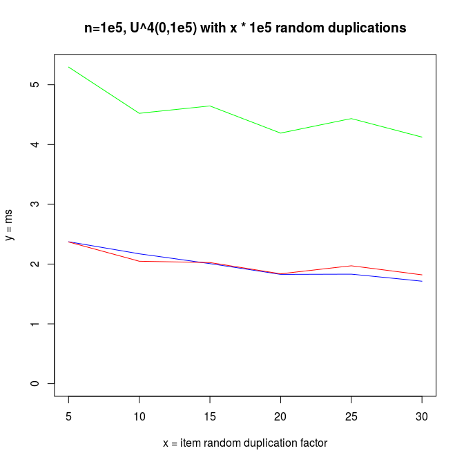
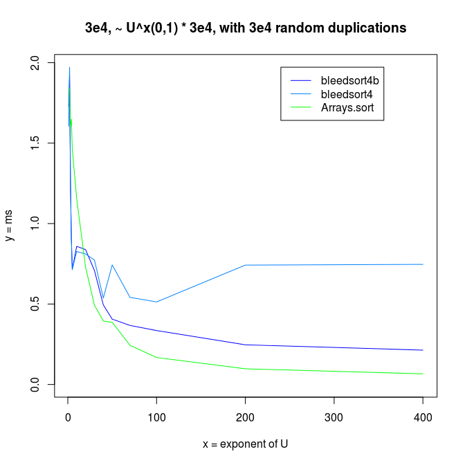
I also made experiments with U^x type distributions, which are plotted next.
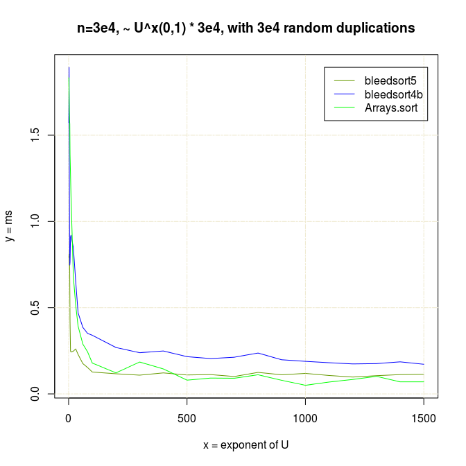
Decreasing arrays, with added noise
Sorting decreasing arrays is one classical benchmark for sort robustness. Some otherwise performant algorithms are reduced to an awful mess by this problem.
Here are some benchmarks from these kinds of tasks.
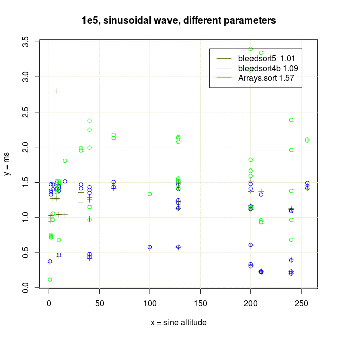
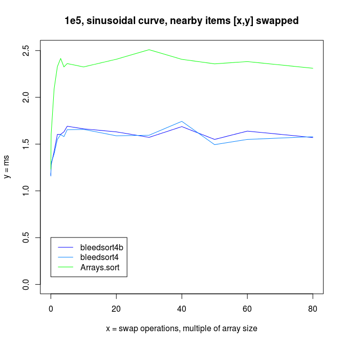
Sinusoidal waves
Java quicksort is especially robust with long monotonously increasing or decreasing runs of values, as it does some preprocessing and then resorts to a very fast, optimized mergesort.
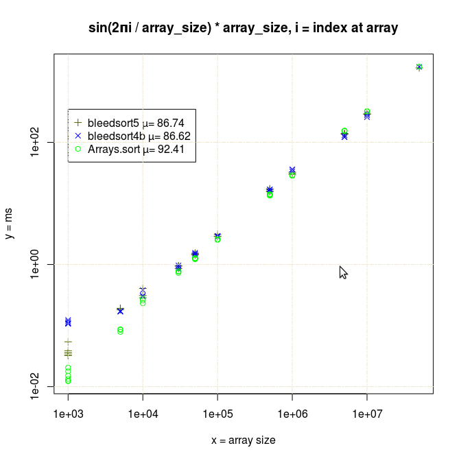
As error (replacements, random copying) increases, the profit from this optimization decreases.
Thanks for your time!
Paavo Toivanen
Experiments, code
paavo.v.toivanen@gmail.com
