Beating Java Sort Performance

17 August 2015

Library sorts in Java 8 are well optimized. For integers and other primitives, Arrays.sort() uses a mixed strategy of two-pivot quicksort, merge sort, and insertion sort that is guided by some heuristics. It is a robust generic solution. Large arrays however have variety that supports even more algorithmic variation. I conducted some experiments to see if my own hastily coded sorts could compete with Java. They did under specific conditions.

Firstly I implemented a classical quicksort. It approximates array median from a sampled mean, using it as an initial pivot.

I cheated a little then and adopted something from Java, making my quicksort fall back to insertion sort with small subarrays. After this I got some sort-times in the same order of magnitude as Java’s. Wild & al suggest that the classical quicksort could perform better than two-pivot quicksort on data with many duplicates. I did not attempt any profiling or bytecode/assembler level optimization. My version would lag behind the highly optimized library routine in most problems.

I had been wanting to test a simple sort algorithm I had in mind. My “Bleedsort” is a distribution sort that takes an array and samples it to estimate a distribution (pardon the double usage here!), then based on that estimate, throws data “in place” into a temp array like in picture 1, then rewrites the original array. This is a preprocessing step to increase order. After that some other sort – in my experiment, my own quicksort. A merge sort might be even better, since it is used by heuristics for highly structured arrays. My experiment is restricted to uniform distributions which are, incidentally, computationally simple.

Bleedsort “bleeds” colliding items towards right, so it sucks with relatively uniform arrays. I sample the target array for an estimate of repetition and skip bleedsort when necessary.

I’m aware that bleedsort does not compete favorably with merge sort (or quicksort) with respect to memory requirements. The temporary array is four times larger than the original. Also Flash sort and other distributive sorts can fare better in this respect.

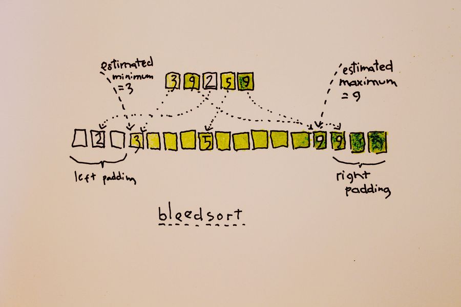Picture 1 illustrates bleedsort (Bleeding Poetry!)

I used JMH for some benchmarks. I kept to int arrays for simplicity. My great success came with arrays of 1000.000 and 10.000.0000 items and uniformly distributed random data. Although my quicksort was somewhat slower on these arrays than Java’s, preprocessing balanced this out nicely (bleedsort followed by own quicksort wins 87ms vs. Java 105ms; 938ms vs. Java 1.144s).

Benchmark                   Mode    Cnt  Score    Error  Units  Corrected
MyBenchmark._1e6U         sample   8512  0.024 ±  0.001   s/op
MyBenchmark._1e7U         sample    985  0.236 ±  0.001   s/op
^^ I timed the generation of target arrays, for correcting benchmarks below

MyBench.int1e6UQuickSort  sample   1641  0.131 ±  0.001   s/op  0.107 ±  0.002
MyBench.int1e6UBleedSort  sample   2410  0.087 ±  0.001   s/op  0.063 ±  0.002
MyBench.int1e6UJavaSort   sample   1978  0.105 ±  0.001   s/op  0.081 ±  0.002

MyBench.int1e7UQuickSort  sample    200  1.483 ±  0.014   s/op  1.247 ±  0.015
MyBench.int1e7UBleedSort  sample    373  0.938 ±  0.009   s/op  0.701 ±  0.010
MyBench.int1e7UJavaSort   sample    200  1.144 ±  0.009   s/op  0.908 ±  0.010

So I won by 20–25% over these datasets, without optimizing my routines. (Edit: 20–25%, not 10–15%. Error in corrected 1e7 values, fixed 2015/08/30)

My sorts didn’t do bad on uniformly increasing datasets of 1000.000 items with 10% or 1% random replacements.

Benchmark                   Mode    Cnt  Score    Error  Units  Corrected
   ._1e6Iwf010            sample  20705  9.701 ±  0.033  ms/op
   ._1e6Iwf001            sample 148693  1.344 ±  0.003  ms/op
^^ Generation of target arrays, for correcting benchmarks again

   .int1e6Iw010BleedSort  sample   4159 49.377 ±  0.571  ms/op 39.68 ±  0.60
   .int1e6Iw010JavaSort   sample   3937 52.139 ±  0.229  ms/op 42.44 ±  0.25
   .int1e6Iw010QuickSort  sample   3899 52.457 ±  0.210  ms/op 42.76 ±  0.23
    ^^ 10% replacements

   .int1e6Iw001BleedSort  sample   6190 32.821 ±  0.219  ms/op 31.48 ±  0.22
   .int1e6Iw001JavaSort   sample   8113 24.910 ±  0.079  ms/op 23.57 ±  0.08
   .int1e6Iw001QuickSort  sample   8653 23.367 ±  0.056  ms/op 22.02 ±  0.06
    ^^ 1%

But they sucked on smallish binomially distributed arrays of 10.000 items (~bin(100, 0.5)). In such arrays an average number of occurences of 50 is 795.9 and of 40, 108.4.

…and they were still twice slower than Arrays.sort() on bigger arrays of 1000.0000 items in ~bin(1e4, 0.5). These arrays have relatively few distinct values (something like 450 distinct of 1e6 total).

Benchmark                   Mode    Cnt  Score    Error  Units  Corrected
   ._1e4bin100    sample 152004  1.316 ±  0.001  ms/op
^^ for correction

   .int1e4bin100BleedSort sample 148681  1.345 ±  0.001  ms/op  0.029 ±  0.002
   .int1e4bin100JavaSort  sample 150864  1.326 ±  0.001  ms/op  0.010 ±  0.002
   .int1e4bin100QuickSort sample 146852  1.362 ±  0.001  ms/op  0.046 ±  0.002

   .int1e6bin1e4BleedSort sample  75344  2.654 ±  0.005  ms/op  -
   .int1e6bin1e4JavaSort  sample 146801  1.361 ±  0.002  ms/op  -
   .int1e6bin1e4QuickSort sample  76467  2.615 ±  0.005  ms/op  -

Smaller (10.000, 100.000) uniformly random arrays were ok but not great.

MyBench.int1e4UBleedSort  sample 216492  0.924 ±  0.001  ms/op  0.683 ±  0.002
MyBench.int1e4UJavaSort   sample 253489  0.789 ±  0.001  ms/op  0.548 ±  0.002
MyBench.int1e4UQuickSort  sample 217394  0.920 ±  0.001  ms/op  0.679 ±  0.002

MyBench.int1e5UBleedSort  sample  18752  0.011 ±  0.001   s/op  0.009 ±  0.002
MyBench.int1e5UJavaSort   sample  22335  0.009 ±  0.001   s/op  0.007 ±  0.002
MyBench.int1e5UQuickSort  sample  18748  0.011 ±  0.001   s/op  0.009 ±  0.002

All in all, I can recommend a distributive sort as an option for moderately big datasets, if memory is not critical.

Finally to give a feel of binomial distributions bin(100, 0.5) and bin(1000, 0.5), here are two random samplings of 100 items (generated with R).

> rbinom(100, 100, 0.5)
  [1] 43 49 51 47 49 59 40 46 46 51 50 49 49 45 50 51 50 49 53 52 45 53 48 56 45
 [26] 47 55 47 53 53 56 41 47 42 51 51 46 49 49 52 46 48 49 50 48 56 54 49 53 52
 [51] 54 48 45 45 50 48 54 49 52 50 48 48 49 45 54 54 50 41 53 45 51 48 53 52 52
 [76] 50 53 47 55 47 60 54 52 56 45 46 54 46 38 43 53 45 62 48 52 52 52 49 52 56

> rbinom(100, 1000, 0.5)
  [1] 515 481 523 519 524 516 498 473 523 514 483 496 458 506 507 491 514 489
 [19] 475 489 485 507 486 523 521 492 502 500 503 501 504 482 518 506 498 525
 [37] 498 491 492 479 506 499 505 497 510 479 504 510 485 488 495 519 522 490
 [55] 517 511 511 488 519 508 475 521 505 493 480 498 490 492 492 476 490 506
 [73] 496 505 521 518 506 509 477 483 509 493 497 501 483 502 470 515 519 509
 [91] 510 496 477 508 506 481 490 511 498 476

Beating Java Sort Performance

Related Posts